Auxiliary Information "Acceleration and transport of relativistic electrons in the parsec-scale jets of the microquasar SS 433"
(H.E.S.S. Collaboration, Science, Vol. 383, pp. 402-406, 2024)
Link to the paper: https://doi.org/10.1126/science.adi2048
Main Text
All plotting scripts make use of the same plot defaults ([PLOT_DEFAULTS.PY]) and Gammapy 0.19
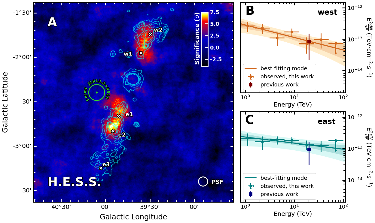
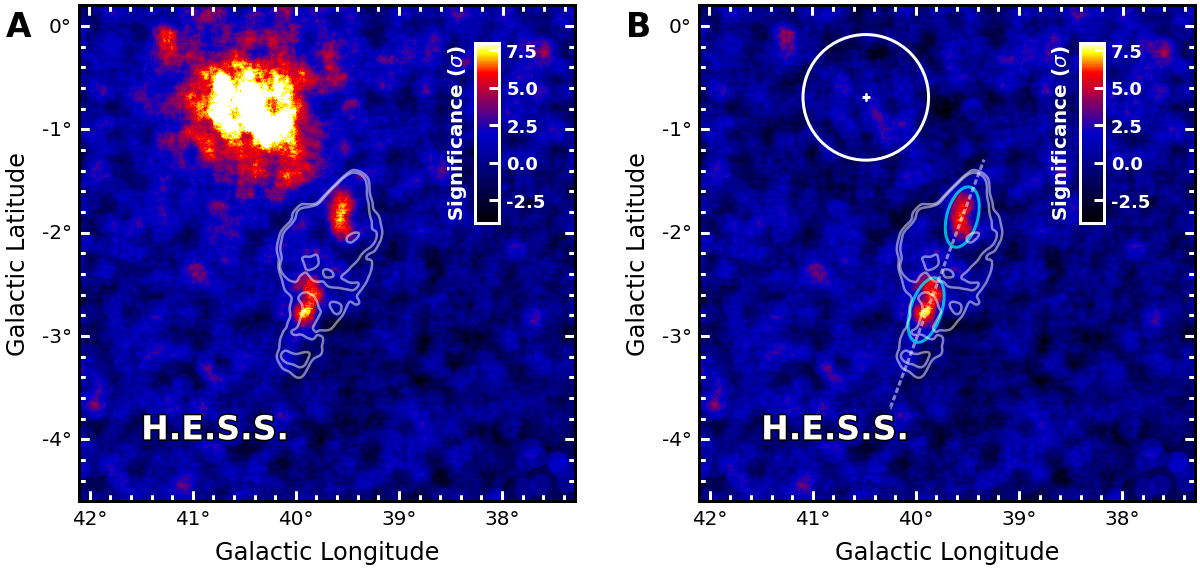
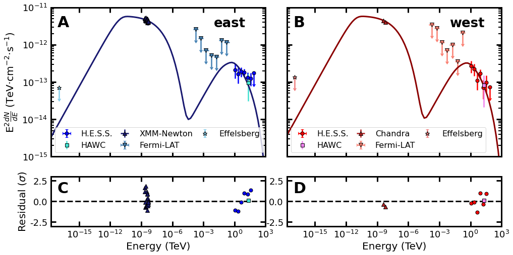
Figure 1: Significance map and spectra of the SS 433 region
Significance/flux maps of the SS 433 region (HESS J1908+063 modeled and subtracted): [SIGNIFICANCE] [FLUX]
Flux points (including systematic uncertainties): [EAST] [WEST]
Count and background maps of the SS 433 region (including HESS J1908+063 contamination): [COUNTS] [BACKGROUND]
Spectral counts, background and response from which the spectral measurements can be derived (see here and here): [EAST] [WEST]
[PDF] [PYTHON_SCRIPT]
| Energy |
Energy Flux East |
Energy Flux Error East |
Energy Flux West |
Energy Flux Error West |
| [TeV] |
[TeV cm-2 s-1] |
[TeV cm-2 s-1] |
[TeV cm-2 s-1] |
[TeV cm-2 s-1] |
| 1.122 |
2.12e-13 |
0.89e-13 |
2.68e-13 |
0.96e-13 |
| 2.239 |
1.66e-13 |
0.76e-13 |
2.26e-13 |
0.80e-13 |
| 4.467 |
1.90e-13 |
0.55e-13 |
1.11e-13 |
0.51e-13 |
| 8.913 |
1.83e-13 |
0.44e-13 |
1.70e-13 |
0.44e-13 |
| 17.783 |
1.32e-13 |
0.44e-13 |
0.72e-13 |
0.39e-13 |
| 35.481 |
1.23e-13 |
0.49e-13 |
0.96e-13 |
0.50e-13 |
| 70.795 |
1.78e-13 (95% UL) |
- |
0.74e-13 (95% UL) |
- |
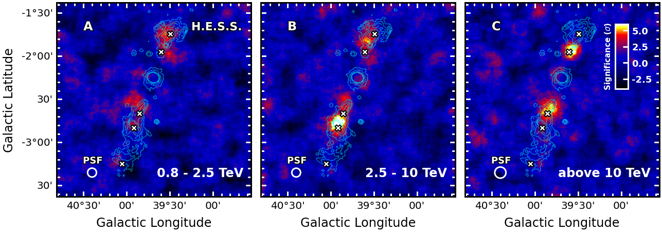
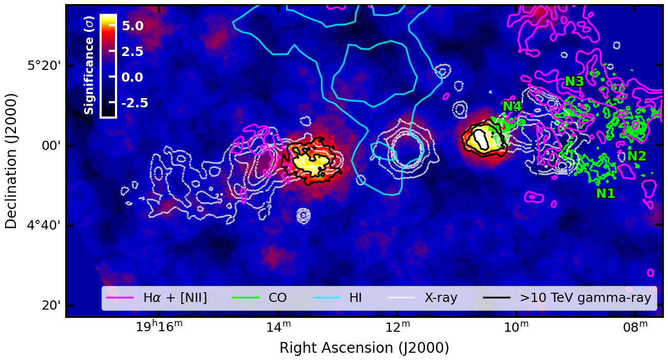
Figure 2: Significance map of the SS 433 region in three energy bands
Significance/flux maps of the SS 433 region in energy bands (HESS J1908+063 modeled and subtracted): [SIGNIFICANCE] [FLUX]
[PDF] [PYTHON_SCRIPT]
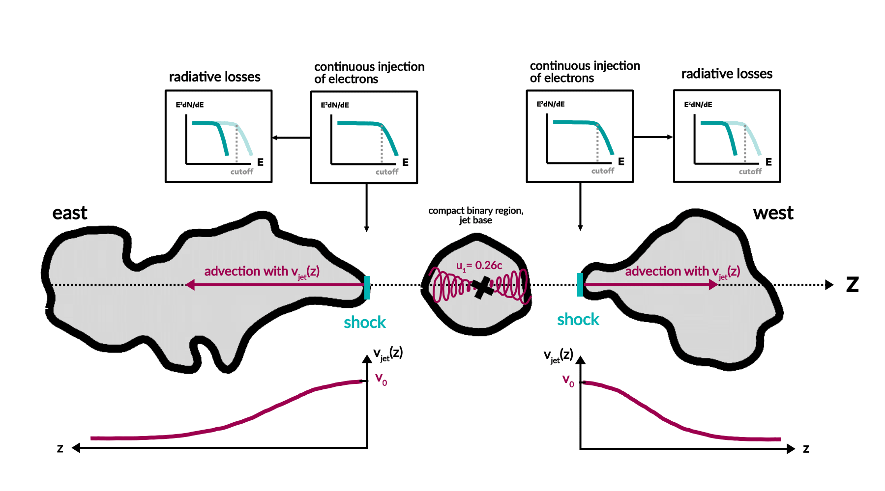
Figure 3: Schematic diagram of the model
[PDF]
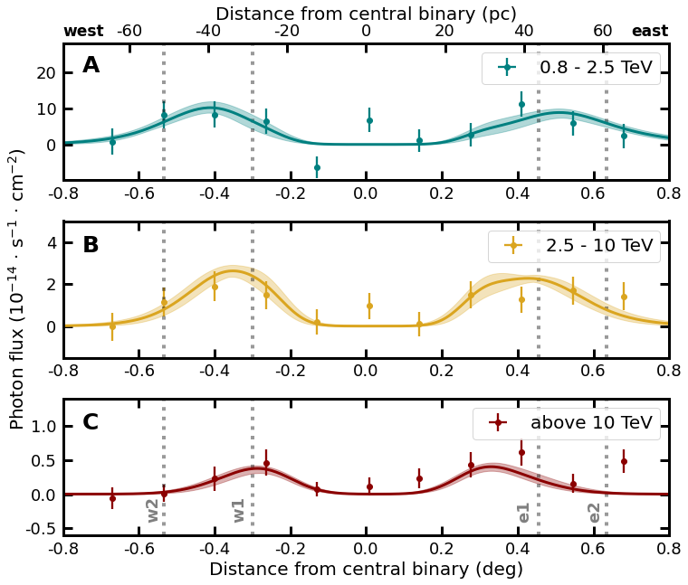
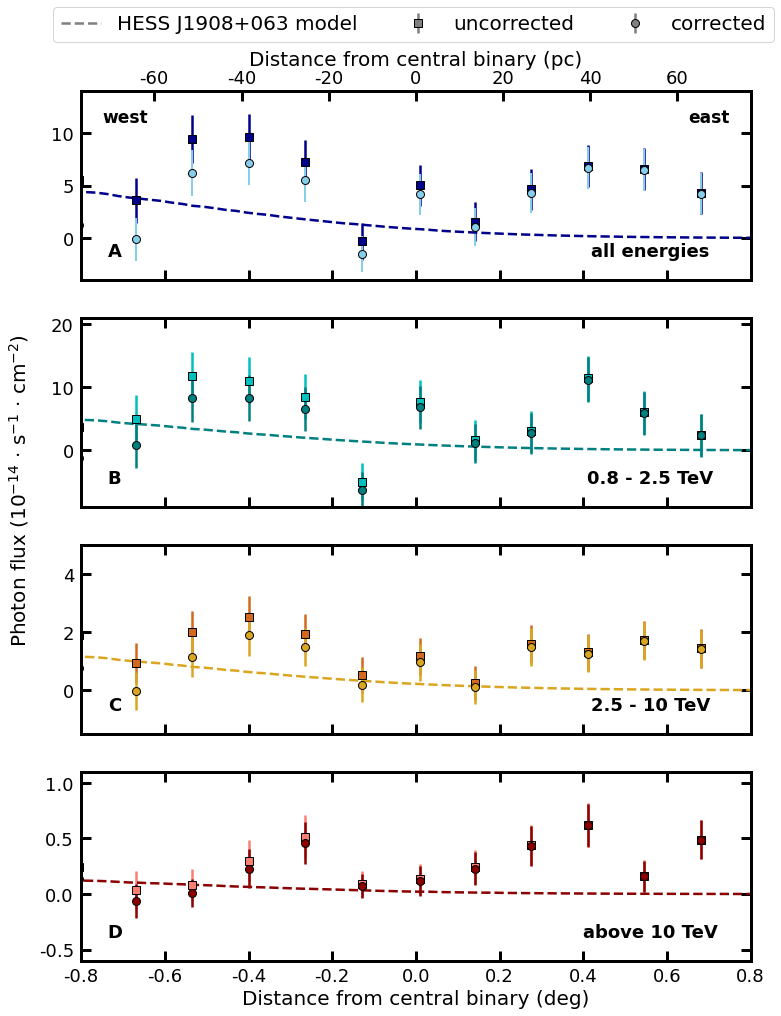
Figure 4: Flux profiles along the jet
Flux points (including systematic uncertainties, HESS J1908 subtracted): [POINTS] [X_AXIS]
Flux ploints in the full energy bands (including systematic uncertainties, HESS J1908 subtracted) : [POINTS]
The code used for the modelling is available via github including examples and resulting files for east and west
(The curves plotted are included here for convenience:
model curves , systematic bands )
[PDF] [PYTHON_SCRIPT]
| Distance from binary |
Photon flux |
Photon flux error |
Photon flux |
Photon flux error |
Photon flux |
Photon flux error |
Photon flux |
Photon flux error |
|
(>0.8 TeV) |
(>0.8 TeV) |
(0.8-2.5 TeV) |
(0.8-2.5 TeV) |
(2.5 - 10 TeV) |
(2.5 - 10 TeV) |
(>10 TeV) |
(>10 TeV) |
| [deg] |
[1e-14 cm-2 s-1] |
[1e-14 cm-2 s-1] |
[1e-14 cm-2 s-1] |
[1e-14 cm-2 s-1] |
[1e-14 cm-2 s-1] |
[1e-14 cm-2 s-1] |
[1e-14 cm-2 s-1] |
[1e-14 cm-2 s-1] |
| -0.670 |
-0.132 |
2.018 |
0.788 |
3.645 |
-0.036 |
0.653 |
-0.0633 |
0.1564 |
| -0.535 |
6.214 |
2.189 |
8.299 |
3.750 |
1.147 |
0.703 |
0.0103 |
0.1284 |
| -0.400 |
7.163 |
2.120 |
8.332 |
3.654 |
1.893 |
0.699 |
0.2295 |
0.1766 |
| -0.265 |
5.489 |
2.015 |
6.525 |
3.497 |
1.487 |
0.665 |
0.4622 |
0.1882 |
| -0.130 |
-1.512 |
1.726 |
-6.355 |
2.938 |
0.189 |
0.597 |
0.0696 |
0.1082 |
| 0.009 |
4.172 |
1.930 |
6.799 |
3.406 |
0.956 |
0.628 |
0.1161 |
0.1353 |
| 0.141 |
1.032 |
1.811 |
1.087 |
3.146 |
0.104 |
0.583 |
0.2287 |
0.1470 |
| 0.276 |
4.307 |
1.919 |
2.669 |
3.262 |
1.494 |
0.650 |
0.4326 |
0.1830 |
| 0.411 |
6.643 |
2.005 |
11.223 |
3.583 |
1.259 |
0.634 |
0.6182 |
0.1952 |
| 0.546 |
6.493 |
1.995 |
5.886 |
3.387 |
1.690 |
0.657 |
0.1585 |
0.1420 |
| 0.681 |
4.234 |
1.957 |
2.354 |
3.342 |
1.423 |
0.657 |
0.4890 |
0.1725 |
Supplementary Material
Figure S1: HESS J1908+063 spectrum
Flux points: [FITS]
Model: [FITS]

[PDF]
| Energy |
Energy Flux |
Energy Flux Error |
| [TeV] |
[TeV cm-2 s-1] |
[TeV cm-2 s-1] |
| 1.000 |
12.037e-12 |
0.851e-12 |
| 1.585 |
12.847e-12 |
0.674e-12 |
| 2.512 |
11.902e-12 |
0.542e-12 |
| 3.981 |
9.764e-12 |
0.505e-12 |
| 6.310 |
8.033e-12 |
0.503e-12 |
| 10.000 |
6.044e-12 |
0.505e-12 |
| 15.849 |
3.691e-12 |
0.494e-12 |
| 25.119 |
2.516e-12 |
0.527e-12 |
| 39.811 |
1.727e-12 |
0.518e-12 |
| 63.096 |
1.426e-12 |
0.502e-12 |
Figure S2: Subtraction of HESS J1908+063
Significance/flux maps of the full field of view (including HESS J1908+063): [SIGNIFICANCE] [FLUX]
Significance/flux maps of the full field of view (HESS J1908+063 modeled and subtracted): [SIGNIFICANCE] [FLUX]
Count and background maps of the full field of view (including HESS J1908+063 contamination): [COUNTS] [BACKGROUND]
[PDF]
Figure S3: Subtraction of HESS J1908+063 (profiles)
Flux points (including systematic uncertainties): [POINTS] [X_AXIS]
[PDF]
Only the "uncorrected" values are listed here, the "corrected" ones are the same as in Figure 4.
| Distance from binary |
Photon flux |
Photon flux error |
Photon flux |
Photon flux error |
Photon flux |
Photon flux error |
Photon flux |
Photon flux error |
|
(>0.8 TeV) |
(>0.8 TeV) |
(0.8-2.5 TeV) |
(0.8-2.5 TeV) |
(2.5 - 10 TeV) |
(2.5 - 10 TeV) |
(>10 TeV) |
(>10 TeV) |
| [deg] |
[1e-14 cm-2 s-1] |
[1e-14 cm-2 s-1] |
[1e-14 cm-2 s-1] |
[1e-14 cm-2 s-1] |
[1e-14 cm-2 s-1] |
[1e-14 cm-2 s-1] |
[1e-14 cm-2 s-1] |
[1e-14 cm-2 s-1] |
| -0.670 |
3.617 |
2.151 |
5.010 |
3.796 |
0.937 |
0.702 |
0.036 |
0.169 |
| -0.535 |
9.441 |
2.288 |
11.736 |
3.862 |
1.990 |
0.738 |
0.079 |
0.143 |
| -0.400 |
9.578 |
2.192 |
11.022 |
3.741 |
2.521 |
0.726 |
0.298 |
0.184 |
| -0.265 |
7.273 |
2.070 |
8.523 |
3.563 |
1.951 |
0.685 |
0.513 |
0.193 |
| -0.130 |
-0.300 |
1.771 |
-4.967 |
2.993 |
0.516 |
0.613 |
0.088 |
0.116 |
| -0.009 |
5.017 |
1.956 |
7.733 |
3.437 |
1.176 |
0.637 |
0.133 |
0.139 |
| 0.141 |
1.567 |
1.828 |
1.672 |
3.167 |
0.247 |
0.59 |
0.243 |
0.149 |
| 0.276 |
4.634 |
1.929 |
3.037 |
3.275 |
1.580 |
0.654 |
0.441 |
0.184 |
| 0.411/td>
| 6.834 |
2.011 |
11.435 |
3.589 |
1.307 |
0.636 |
0.624 |
0.196 |
| 0.546 |
6.595 |
1.998 |
5.999 |
3.391 |
1.716 |
0.658 |
0.161 |
0.142 |
| 0.681 |
4.288 |
1.959 |
2.415 |
3.344 |
1.437 |
0.658 |
0.49 |
0.173 |
Figure S4: Excluded significance distribution
Can be derived from significance maps linked above
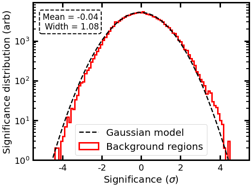
[PDF]
Figure S5: Excluded significance distribution
Can be derived from significance maps linked above
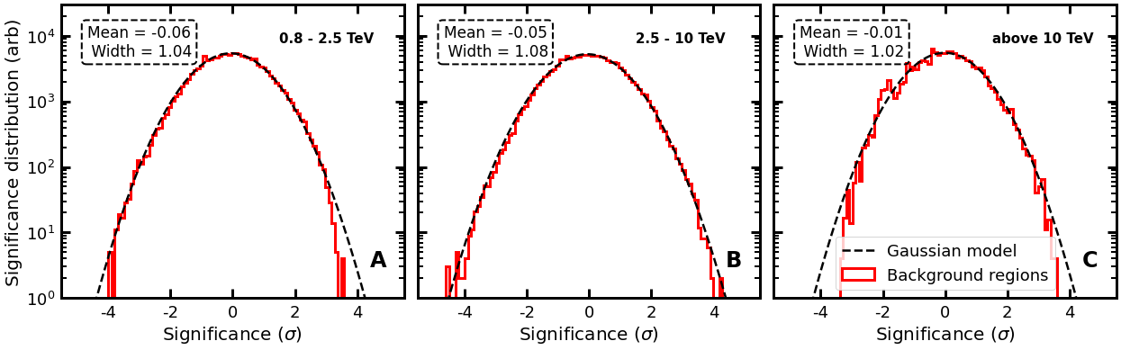
[PDF]
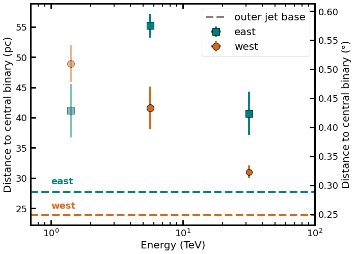
Figure S6: Distance of peak gamma-ray emission from central binary
Values can be found in Table S4 in the paper
[PDF]
Figure S7: Upper limits from the central and e3 regions
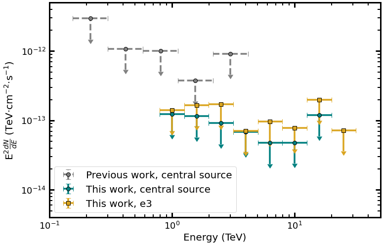
[PDF]
| Energy |
UL center (95%) |
UL e3 (95%) |
| [TeV] |
[TeV cm-2 s-1] |
[TeV cm-2 s-1] |
| 1 |
1.239e-13 |
1.403e-13 |
| 1.585 |
1.149e-13 |
1.664e-13 |
| 2.512 |
0.913e-13 |
1.702e-13 |
| 3.981 |
0.68e-13 |
0.705e-13 |
| 6.310 |
0.474e-13 |
0.969e-13 |
| 10.000 |
0.480e-13 |
0.775e-13 |
| 15.849 |
1.188e-13 |
1.988e-13 |
| 25.119 |
- |
0.723e-13 |
Figure S8: X-ray flux points
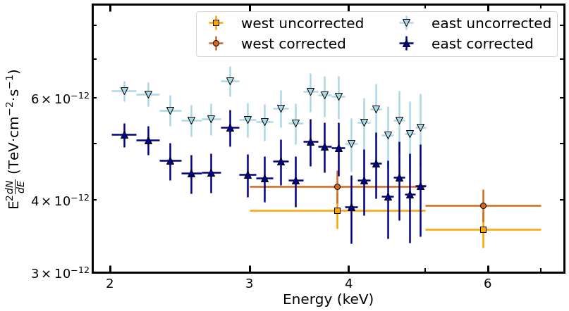
[PDF]
Figure S9: Radiation fields
Number density (in cgs) at the location of the [central source], the [eastern jet] and the [western jet]
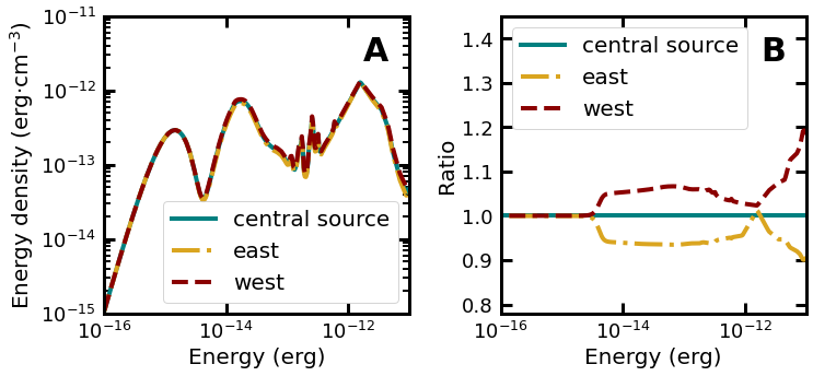
[PDF]
Figure S10: Multi-wavelength SED
H.E.S.S. flux points are the same as in Figure 1
[PDF]
Figure S11: Model dependence on assumed injection time
H.E.S.S. flux points are the same as in Figure 1
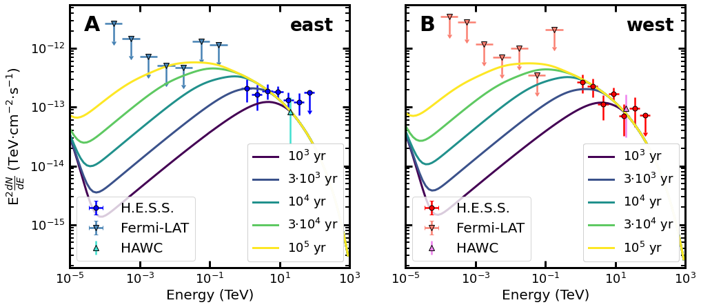
[PDF]
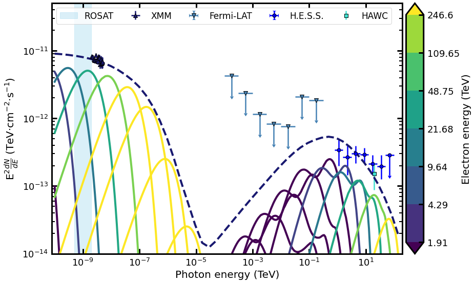
Figure S12: Contribution to the model of electrons with different energies
H.E.S.S. flux points are the same as in Figure 1
[PDF]
Figure S13: Timescales
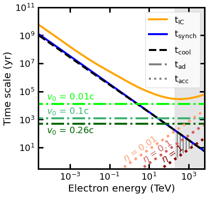
[PDF]
Figure S14: Velocity profiles
For the [eastern jet] and the [western jet]
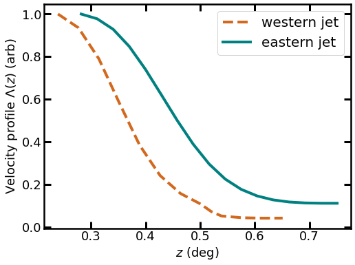
[PDF]
Figure S15: Velocity systematics
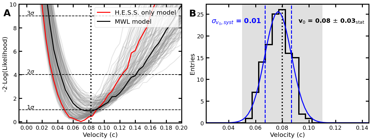
[PDF]
Figure S16: Possible hadronic targets
Significance map is the same as in Figure 2
[PDF]
Collaboration Acknowledgement
The support of the Namibian authorities and of the University of
Namibia in facilitating the construction and operation of H.E.S.S.
is gratefully acknowledged, as is the support by the German
Ministry for Education and Research (BMBF), the Max Planck Society,
the German Research Foundation (DFG), the Helmholtz Association,
the Alexander von Humboldt Foundation, the French Ministry of
Higher Education, Research and Innovation, the Centre National de
la Recherche Scientifique (CNRS/IN2P3 and CNRS/INSU), the
Commissariat à l’énergie atomique et aux énergies alternatives
(CEA), the U.K. Science and Technology Facilities Council (STFC),
the Irish Research Council (IRC) and the Science Foundation Ireland
(SFI), the Knut and Alice Wallenberg Foundation, the Polish
Ministry of Education and Science, agreement no. 2021/WK/06, the
South African Department of Science and Technology and National
Research Foundation, the University of Namibia, the National
Commission on Research, Science & Technology of Namibia (NCRST),
the Austrian Federal Ministry of Education, Science and Research
and the Austrian Science Fund (FWF), the Australian Research
Council (ARC), the Japan Society for the Promotion of Science, the
University of Amsterdam and the Science Committee of Armenia grant
21AG-1C085. We appreciate the excellent work of the technical
support staff in Berlin, Zeuthen, Heidelberg, Palaiseau, Paris,
Saclay, Tübingen and in Namibia in the construction and operation
of the equipment. This work benefited from services provided by the
H.E.S.S. Virtual Organisation, supported by the national resource
providers of the EGI Federation.